Automatic differentiation (AD) has been a hot topic now with the bloom of neural networks. Automatic differentiation relies on computation of gradients of complicated operations by applying chain rule sequentially to each small operations (e.g. addition, subtraction, multiplication, division), which plays a big part in backpropagation for training a neural network.
Speaking of training neural networks, there are several high level python libraries that support building and training neural network models, such as PyTorch from Facebook and TensorFlow from Google. From my limited experience, tensorflow tends to be faster but not as flexible because it compiles the computational graph. On the other hand, pytorch is relying on dynamic graphs, and “pythonic”-enough to let you print/inspect/debug intermediate results from any layers of the neural networks with a numpy-like API.
Now, here comes JAX, a low level library from google (again). JAX can almost be used in place of numpy, but with gradient easily computed from the functions and can be translate to multi CPU, GPU or TPU codes easily under the hood. I think it has a great potential to be used as underlying codes in neural network framework libraries, such as Flax.
So in this post, I’m going to experiment using JAX in the most simplistic way: Linear model or, more fancy, a single neuron in a neural network. I will be write a Batch Gradient Descent function for solving linear model with minibatches.
So the components that we need are:
But first, lets import everything:
import jax.numpy as np
import jax
import numpy as onp
import matplotlib.pyplot as plt
import logging
logging.basicConfig(level=logging.INFO)
logger = logging.getLogger('JAX SGD')
I’ll just make a bootstrapping object that takes in the input data, and return a generator that generates indices for the minibatches.
class Bootstrap:
    def __init__(self, seed=123):
        '''
        boostrap 1d array
        usage:
        xs = np.arange(100)
        bs = Bootstrap(seed=123)
        for idx in bs.bootstrap(xs, group_size=50, n_boots=10):
            print(xs[idx].mean())
        '''
        self.rng = onp.random.RandomState(seed)

    def bootstrap(self, xs, group_size=100, n_boots = 100):
        '''
        input:
            xs: 1d np.array
            group_size: number of values in each bootstrap iteration
            n_boots: how many bootstrap groups
        output:
            iterator: bootstrapped
        '''
        xs = onp.array(xs)
        total_size = xs.shape[0]
        logger.info('Total size for bootstrap: %i' %total_size)
        if group_size > total_size:
            raise ValueError('Group size > input array size')

        for i in range(n_boots):
            idx = self.rng.randint(0, total_size, group_size)
            yield idx
The loss function I use here is just the root mean square loss function, and we can speed it up jax.jit:
@jax.jit
def loss_function(params, x, y):
    '''
    Root mean square loss function:

    input:
        - params: a list [w, b] where w are the weights and b is the bias term
        - x: input data for training (np.array)
        - y: target data (np.array)

    return:
        - RMSE value (float)
    '''
    predict = x.dot(params[0]) + params[1]
    deviation = y - predict
    squared_deviation = deviation ** 2
    mean_squared_deviation = squared_deviation.mean()
    return np.sqrt(mean_squared_deviation)
So to fit a model:
__InitParams__.loss_gradient function, which is automatically generated from doing jax.grad(loss_function).__update__ function. There are of course better optimizer for updating weights, such as Adam. But here for simplicity, we will use the easiest one, which the parameters are updated with new_value = old_value - learning rate * gradient.class SGD():
'''
This is a linear model sovler using minibatch stochastic gradient descent
usage:
# some test data
X = 10 * onp.random.random((1000,2))
y = X.dot([3,4]) + onp.random.random(1000) + 5
#model fitting
lm = SGD(n_epoch=10000, learning_rate=0.001)
lm.fit(X,y)
'''
def __init__(self,
learning_rate = 1e-3,
n_epoch = 1000):
'''
input:
- learning_rate: learning rate for updating the parameters
- n_epoch: how many steps to train for
'''
self.learning_rate = learning_rate
self.n_epoch = n_epoch
self.losses = onp.zeros(n_epoch)
self.coef_ = None
self.intercept_ = None
self.gradients = None
self._iter = 0
def fit(self, X, y):
if X.ndim != 2:
raise ValueError('X must have 2 dimension')
self.__InitParams__(X)
bootstrap = Bootstrap()
subsets = bootstrap.bootstrap(X, group_size=100, n_boots = self.n_epoch)
loss_gradient = jax.grad(loss_function)
for i in range(self.n_epoch):
self._iter += 1
train_idx = next(subsets)
X_train, y_train = X[train_idx], y[train_idx]
loss = loss_function([self.coef_, self.intercept_], X_train, y_train)
self.losses[i] = loss
self.gradients = loss_gradient([self.coef_, self.intercept_], X_train, y_train)
self.__update__()
if self._iter % (self.n_epoch//10) == 0:
logger.info('%i epoch - Loss: %.2f' %(self._iter, loss))
def predict(self, X):
return X.dot(self.coef_) + self.intercept_
def __InitParams__(self, X):
# initialize weights and bias terms
self.coef_ = onp.random.randn(X.shape[1])
self.intercept_ = onp.random.randn(1)
self._iter = 0
def __update__(self):
# update weight and bias terms with graidents
# gradient[0]: gradients for coefficients
# gradient[1]: gradients for the bias term
self.coef_ -= self.gradients[0] * self.learning_rate
self.intercept_ -= self.gradients[1] * self.learning_rate
Now, let’s generate some data and test if this SGD works! We will make some test data following: $y$ = 3$X_1$ + 4$X_2$4 + 5
X = 10 * onp.random.random((1000,2))
y = X.dot([3,4]) + onp.random.random(1000) + 5
And let’s fit the model with 10000 steps and a learning rate of 0.001
lm = SGD(n_epoch=5000, learning_rate=0.01)
lm.fit(X,y)
INFO:JAX SGD:Total size for bootstrap: 1000
/home/wckdouglas/miniconda3/lib/python3.6/site-packages/jax/lib/xla_bridge.py:125: UserWarning: No GPU/TPU found, falling back to CPU.
warnings.warn('No GPU/TPU found, falling back to CPU.')
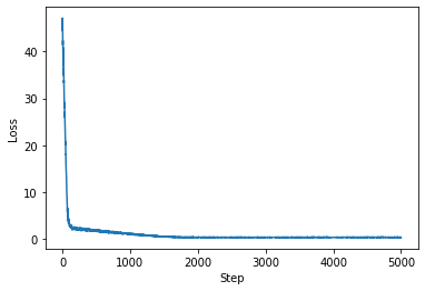
INFO:JAX SGD:500 epoch - Loss: 1.66
INFO:JAX SGD:1000 epoch - Loss: 1.03
INFO:JAX SGD:1500 epoch - Loss: 0.46
INFO:JAX SGD:2000 epoch - Loss: 0.26
INFO:JAX SGD:2500 epoch - Loss: 0.27
INFO:JAX SGD:3000 epoch - Loss: 0.30
INFO:JAX SGD:3500 epoch - Loss: 0.27
INFO:JAX SGD:4000 epoch - Loss: 0.29
INFO:JAX SGD:4500 epoch - Loss: 0.32
INFO:JAX SGD:5000 epoch - Loss: 0.28
Plotting the loss at each step:
plt.plot(lm.losses)
plt.xlabel('Step')
plt.ylabel('Loss')
Text(0, 0.5, 'Loss')
lm.coef_, lm.intercept_
(DeviceArray([2.9833608, 3.9956608], dtype=float32),
 DeviceArray([5.4867635], dtype=float32))
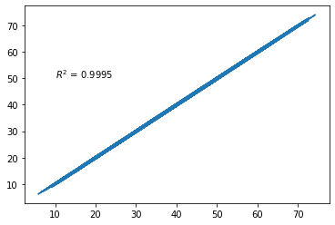
from sklearn.metrics import r2_score
plt.plot(y, lm.predict(X))
plt.text(10,50, '$R^2$ = %.4f' %r2_score(y, lm.predict(X)))
Text(10, 50, '$R^2$ = 0.9995')
And here’s a great SciPy talk for JAX from Jake Vanderplas.
